Introduction

I have been exploring Expected Parrot—a framework for simulating participant data with LLMs—to replicate the results of my experimental studies. I think there is a lot of potential for these sorts of tools to give researchers preliminary insights into the likely effects of their experimental studies when using power analyses or other methods for determining appropriate sample sizes.

As an initial test, I wanted to look at a main effect study from my recent paper on “Retributive Philanthropy”. Here, we used some scenario studies to assess the impact of volitional and non-volitional wrongdoing on willingness to make retributive donations. The underlying theory here is that wrongdoing that is willful and/or actively desired by the wrongdoer tells you much more about their character than wrongdoing which is accidental.

The specific manipulation we used was a real story of a professor who said a Chinese word that sounds similar to the N-word to his students. This was manipulated to be either presented as-is, or with an alternative story where the professor actually said the N-word to students. Participants were then presented with the opportunity to make a retributive donation, with willingness to donate rated on a 7-point scale.

Simulation

There are a few relatively simple steps I took to begin simulating this data: library setup, scenario and question setup, model setup, and participant setup. Note that this is all done in Python, as there isn’t an equivalent R package to do this (yet).

Library setup

First, I needed to load in the edsl library as well as another supporting library:

from edsl import QuestionMultipleChoice, QuestionFreeText, QuestionLinearScale, \
    Survey, FileStore, Scenario, ScenarioList, AgentList, Agent, Model, ModelList
from itertools import product

Scenario and question setup

Next, I pre-set the scenario manipulation as well as the questions used in our study with the edsl package:

scenarios = ScenarioList.from_source("pdf", "stimuli/intentional.pdf") + \
ScenarioList.from_source("pdf", "stimuli/unintentional.pdf")

stimuli = QuestionFreeText(
  question_name = "stimuli",
  question_text = "How do you feel about this story: {{ scenario.text }}"
)

nmj_1 = QuestionLinearScale(
  question_name = "nmj_1",
  question_text = "I believe Professor Gerber harmed his Black students",
  question_options = [1,2,3,4,5,6,7,],
  option_labels = {1:"Strongly disagree", 7:"Strongly agree"},
  include_comment = False
)

nmj_2 = QuestionLinearScale(
  question_name = "nmj_2",
  question_text = "I believe Professor Gerber intended to harm his Black students",
  question_options = [1,2,3,4,5,6,7,],
  option_labels = {1:"Strongly disagree", 7:"Strongly agree"},
  include_comment = False
)

nmj_3 = QuestionLinearScale(
  question_name = "nmj_3",
  question_text = "I blame Professor Gerber for harming his Black students",
  question_options = [1,2,3,4,5,6,7,],
  option_labels = {1:"Strongly disagree", 7:"Strongly agree"},
  include_comment = False
)

dv = QuestionLinearScale(
  question_name = "dv",
  question_text = "In response to this incident, the Kentucky Antiracist Students Alliance (KASA) is raising funds to support those harmed by the professor's speech. For each donation, KASA promises to send a letter calling for the professor's dismissal. Please rate your likelihood of donating to KASA below:",
  question_options = [1,2,3,4,5,6,7,],
  option_labels = {1:"Extremely unlikely", 7:"Extremely likely"},
  include_comment = False
)

Model setup

I then set up this process to use a range of different LLM models. Ideally, these results will not depend on the idiosyncracies of a single model, so I use a range of models to generate the results. This will help me understand how the results vary (or ideally, remain consistent) across different models. Right now, I am using several models from Google, Anthropic, and Mistral. These are the cheapest models available from each provider (based on this listed curated by ExpectedParrot: https://www.expectedparrot.com/models), which should be sufficient for this study. Presumably, more expensive models will produce better results, but I am not interested in that right now.

I am also setting models to have a temperature of 1.0. Expected Parrot appears to have a default temperature value of 0.5, but given that I will be replicating responses many times, I want to maximize some more randomness in model results.

models = ModelList([
  Model("gemini-1.5-flash-8b", service_name = "google", temperature = 1.0),
  Model("claude-3-haiku-20240307", service_name = "anthropic", temperature = 1.0),
  Model("mistral.mistral-7b-instruct-v0:2", service_name = "bedrock", temperature = 1.0),
])

Participant setup

I next wanted to get a relatively random assortment of participants for this analysis. The code below simulates a rough distribution of genders, ages, and other demigraphic characteristics to make each model’s results more robust.

Right now, what this code does is provide every combination of each option for age, gender, nationality, and political views. Realistically, I would want to include more nationalities, more gender diversity, have an age curve more broadly representative of the population and/or Prolific’s user base, and have better weighting of different combinations (e.g., men are more conservative than women, whereas this code assumes equal representation).

However, for the sake of simplicity, I will use this smaller set of agents:

ages = [20, 25, 30, 35, 40, 45]
genders = ["Male", "Female"]
nationalities = ["American", "Canadian"]
political_views = ["Conservative", "Liberal", "Moderate", "Progressive"]

agents = AgentList(
    Agent(traits={"age": age, "gender": gender, "nationality": nationality, "politics": politics})
    for age, gender, nationality, politics in product(ages, genders, nationalities, political_views)
)

Running the survey

Finally, I can run the survey and save all data:

survey = Survey(questions = [stimuli, nmj_1, nmj_2, nmj_3, dv])
survey = survey.set_full_memory_mode()

results = survey.by(scenarios).by(agents).by(models).run()

results.to_csv("results/blended/full.csv")

results.select("filename", "model", "age", "gender", "nationality", "politics", 
               "generated_tokens.nmj_1_generated_tokens", 
               "generated_tokens.nmj_2_generated_tokens", 
               "generated_tokens.nmj_3_generated_tokens", 
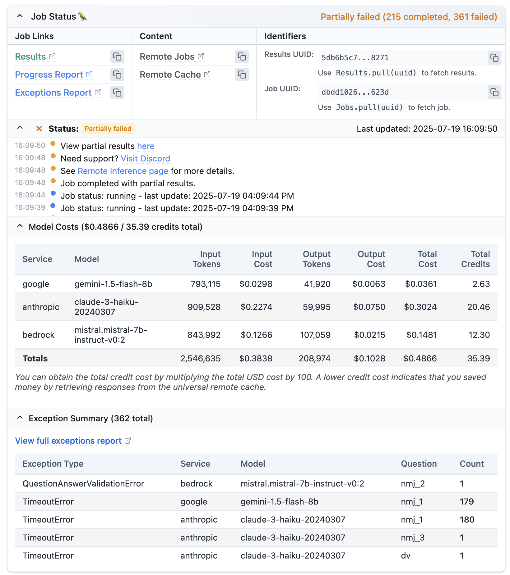
               "generated_tokens.dv_generated_tokens").to_csv("results/blended/reduced.csv")

Here is what running the model looks like:

Now that the simulated data is generated, I can then analyze the results and compare them to what we found in our study of real participants.

Comparison

I generally prefer working with R, so I will load the data in and analyze it using R instead of Python. Here’s some quick code to load in the simulated data and report the results of a between-conditions t-test:

library(here)
library(tidyverse)

data <- read_csv(here("blog", "expected_parrot", "results", "google", "reduced.csv"))

data <- data |>
  mutate(across(.cols = matches("nmj|dv"),
                .fns = ~ as.numeric(str_extract(as.character(.x), "\\d")))) 

names(data) <- names(data) |>
  str_replace_all("generated_tokens\\.", "") %>%
  str_replace_all("_generated_tokens", "")

t.test(data[data$scenario.filename == "intentional.pdf",]$dv,
data[data$scenario.filename == "unintentional.pdf",]$dv)


    Welch Two Sample t-test

data:  data[data$scenario.filename == "intentional.pdf", ]$dv and data[data$scenario.filename == "unintentional.pdf", ]$dv
t = 5.5398, df = 361.49, p-value = 5.84e-08
alternative hypothesis: true difference in means is not equal to 0
95 percent confidence interval:
 0.4255307 0.8939137
sample estimates:
mean of x mean of y 
 2.690972  2.031250

These results look like very similar results to what was reported in the paper! The mean willingness to retributively donate in the intentional condition was almost exactly the same for the real (M = 2.67) and simulated data (M = 2.69); the mean willingness to retributively donate in the unintentional condition was very close for both the real (M = 1.83) and simulated data (M = 2.03) as well. The statistical tests were both significant as well (though these two studies differed in overall sample size):

Real: t(1109.2) = 8.40, (p < .001)
Simulated: t(361.49) = 5.54, (p < .001)

(Note that for the purpose of this analysis, I am only showing the output of Google’s gemini 1.5 flash modelm but the results I am sharing are consistent across the different models I tested.)

In short, it looks like for this sort of study, LLM-based simulations work very well! I can imagine a lot of use-cases for this. In particular, I think power analyses could be greatly helped by LLM-based simulation: right now, power analysis often requires the researcher to either guess what an effect might be or identify what a minimally interesting effect size might be in order to calculate the necessary sample for an experiment. If these models work well, I could see researchers using them to more easily simulate data prior to power analysis in order to get a better grounding for their likely effect sizes.

Conclusion

This was a small test of using LLMs to simulate experimental data. This is a growing area of research that a lot of behavioral scientists are paying attention to, and noting areas where LLM-simulated data converges and diverges from “real” studies will be important as our discipline considers how best to use this information in the design, execution, and replication of experimental studies. Hopefully this was useful to anybody interested in trying this method out for themselves!